User Analysis on reshare cascades about COVID-19
We demonstrate in this blog post a tutorial on applying the tools for analyzing online information diffusions about Twitter users, birdspotter and evently.
Dataset
In this tutorial, we apply two tools for analyzing Twitter users, on a COVID-19 retweet dataset. The dataset
is curated by Chen, et al. One can obtain a copy of the tweet IDs from
their project. We
only use the 31st of Janury sample of the whole dataset for
demonstration purpose. The tweets can be recovered by hydration
from their IDs. We note that some tweets might have been deleted and in
the end we manage to get 69.2% (1,489,877) of the original tweets.
Tools
While BirdSpotter captures the social influence and botness of Twitter
users, evently specifically models the temporal dynamics of online
information diffusion. We leverage information provided by the tools to
study the users in the COVID19 dataset.
library(evently)
library(reticulate)
birdspotter <- import('birdspotter')
Preprocessing tweets
At this step, we seek to extract diffusion cascades from the COVID-19
dataset for analyzing user influence and botness. A diffusion cascade
consist of an initial tweet posted by a Twitter user and followed then
by a sereis of retweets. A function provided by evently allows one to
obtain cascades from JSON formatted raw tweets. On the other hand, we
initialize a BirdSpotter instance and compute the influence and
botness scores for all users in the
dataset.
cascades <- parse_raw_tweets_to_cascades('corona_2020_01_31.jsonl', keep_user = T, keep_absolute_time = T)
bs <- birdspotter$BirdSpotter('corona_2020_01_31.jsonl')
labeled_users <- bs$getLabeledUsers()[, c('user_id', 'botness', 'influence')]
As we cannot publish corona_2020_01_31.jsonl due to Twitter TOC, we
have stored the results and load them below
load('corona_2020_01_31.rda')
labeled_users <- read.csv('corona_31_botness_influence.csv', stringsAsFactors = F,
                          colClasses=c("character",rep("numeric",3)))
We note that all user IDs have been encrypted. After obtaining the results, let’s first conduct some simple measurements on users and cascades.
library(ggplot2)
# check the density of these two values
mean_bot <- mean(labeled_users$botness, na.rm = T)
ggplot(labeled_users, aes(botness)) +
  stat_density(geom = 'line') +
  geom_vline(xintercept = mean_bot, linetype=2, color = 'red') +
  geom_text(data=data.frame(), aes(x = mean_bot, y = 2, label= sprintf('mean: %s', round(mean_bot, 2))), color= 'red', angle=90, vjust=-0.11)

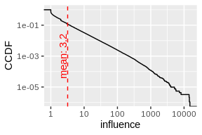
mean_inf <- mean(labeled_users$influence)
ggplot(labeled_users) +
  stat_ecdf(aes(influence, 1 - ..y..)) +
  scale_x_log10() +
  scale_y_log10() +
  ylab('CCDF') +
  geom_vline(xintercept = mean_inf, linetype=2, color = 'red') +geom_text(data=data.frame(), aes(x = mean_inf, y = 1e-3, label= sprintf('mean: %s', round(mean_inf, 2))), color= 'red', angle=90, vjust=-0.11)
## Warning: Transformation introduced infinite values in continuous y-axis
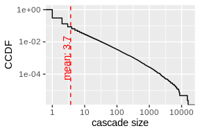
mean_value <- mean(sapply(cascades, nrow))
ggplot(data.frame(size = sapply(cascades, nrow))) +
  stat_ecdf(aes(size, 1 - ..y..)) +
  scale_x_log10() + scale_y_log10() +
  geom_vline(xintercept = mean_value, linetype=2, color = 'red') +
  geom_text(data=data.frame(), aes(x = mean_value, y = 1e-3, label= sprintf('mean: %s', round(mean_value, 2))), color= 'red', angle=90, vjust=-0.11) +
  xlab('cascade size') +
  ylab('CCDF')
## Warning: Transformation introduced infinite values in continuous y-axis
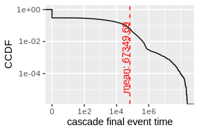
mean_value2 <- mean(sapply(cascades, function(c) c$time[nrow(c)]))
ggplot(data.frame(time = sapply(cascades, function(c) c$time[nrow(c)]))) +
  stat_ecdf(aes(time, 1 - ..y..)) +
  scale_x_continuous(trans = 'log1p', breaks = c(0, 100, 10000, 1000000), labels = c('0', '1e2', '1e4', '1e6')) +
  scale_y_log10() +
  geom_vline(xintercept = mean_value2, linetype=2, color = 'red') +
  geom_text(data=data.frame(), aes(x = mean_value2, y = 1e-3, label= sprintf('mean: %s', round(mean_value2, 2))), color= 'red', angle=90, vjust=-0.11) +
  xlab('cascade final event time')+
  ylab('CCDF')
## Warning: Transformation introduced infinite values in continuous y-axis
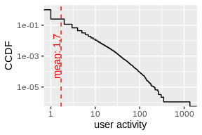
mean_value <- mean(labeled_users$activity)
ggplot(data.frame(size = labeled_users$activity)) +
   stat_ecdf(aes(size, 1 - ..y..)) +
   scale_x_log10() +
   scale_y_log10() +
   geom_vline(xintercept = mean_value, linetype=2, color = 'red') +
   geom_text(data=data.frame(), aes(x = mean_value, y = 1e-3, label= sprintf('mean: %s', round(mean_value, 2))), color= 'red', angle=90, vjust=-0.11) + xlab('user activity')+ ylab('CCDF')
## Warning: Transformation introduced infinite values in continuous y-axis
Retrain the bot detector
If one find the botness scores are not accurate, birdspotter provides
a relabeling tool and a retrain API to learn from the given relabeled
dataset
# output a file for mannual labeling
bs$getBotAnnotationTemplate('users_to_label.csv')
# Once annotated the botness detector can be trained with
bs$trainClassifierModel('users_to_label.csv')
Fit user posted cacsades with evently
We model a group of cascades initiated by a particular user jointly and treat the fitted model as a characterization of the user. In this example, we select two users for comparison.
selected_users <- c('369686755237813560', '174266868073402929')

# fit Hawkes process on cascades initiated by the selected users
user_cascades_fitted <- lapply(selected_users, function(user) {
  # select cascades that are initiated by the "selected_user"
  selected_cascades <- Filter(function(cascade) cascade$user[[1]] == user, cascades)
  # obtain the observation times;
  # note 1580515200 is 1st Feb when the observation stopped
  # as we only observed until the end of 31st Jan
  times <- 1580515200 - sapply(selected_cascades, function(cas) cas$absolute_time[1])
  # fit a model on the selected cascades;
  fit_series(data = selected_cascades, model_type = 'mPL', observation_time = times, cores = 10)
})
user_cascades_SEISMIC_fitted <- lapply(selected_users, function(user) {
  selected_cascades <- Filter(function(cascade) cascade$user[[1]] == user, cascades)
  times <- 1580515200 - sapply(selected_cascades, function(cas) cas$absolute_time[1])
  fit_series(data = selected_cascades, model_type = 'SEISMIC',
             observation_time = times)
})
# check the fitted kernel functions
plot_kernel_function(user_cascades_fitted) +
  scale_color_discrete(labels = c("@BobOngHugots", "@Jaefans_Global"))
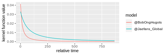
The plot shows the fitted kernel functions of these two users which reflect their time-decaying influence of attracting followers to reshare their posts. We then demonstrate how to simulate new cascades
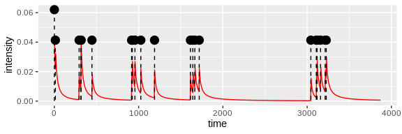
set.seed(134841)
user_magnitude <- Filter(function(cascade) cascade$user[[1]] == selected_users[[1]], cascades)[[1]]$magnitude[1]
# simulate a new cascade from @BobOngHugots
sim_cascade <- generate_series(user_cascades_fitted[[1]], M = user_magnitude)
plot_event_series(cascade = sim_cascade, model = user_cascades_fitted[[1]])
selected_cascade <- Filter(function(cascade) cascade$user[1] == selected_users[[1]], cascades)[[1]]
selected_time <- user_cascades_fitted[[1]]$observation_time[1]
# simulate a cascade with a "selected_cascade" from @BobOngHugots
sim_cascade <- generate_series(user_cascades_fitted[[1]], M = user_magnitude,
                               init_history = selected_cascade)
sprintf('%s new events simulated after cascade',
        nrow(sim_cascade[[1]]) - nrow(selected_cascade))
## [1] "25 new events simulated after cascade"
predict_final_popularity(user_cascades_fitted[[1]],
                         selected_cascade, selected_time)
## [1] 458.303
# predict with SEISMIC model, assume we have fitted the SEISMIC model
predict_final_popularity(user_cascades_SEISMIC_fitted[[1]],
                         selected_cascade, selected_time)
## [1] 729.923
get_branching_factor(user_cascades_fitted[[1]])
## [1] 0.7681281
get_viral_score(user_cascades_fitted[[1]])
## [1] 7.407763
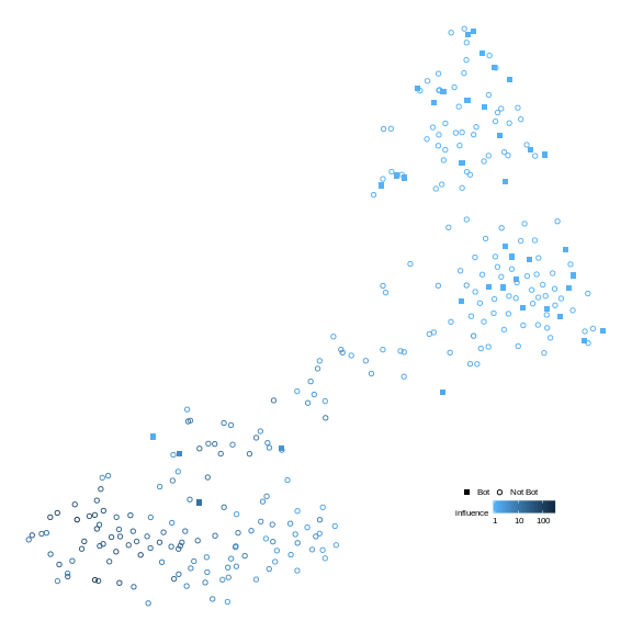
Visualize users in a latent space
We show a visualization of top 300 users posted most tweets using the
features returned by evently along with the botness and influence
scores from birdspotter.
# obtain observation times here again
times <- 1580515200 - sapply(cascades, function(cas) cas$absolute_time[1])
# indicate the grouping of each cascade with the user who started the cascade
names(cascades) <- sapply(cascades, function(cas) cas$user[1])
# fit Hawkes processes on all cascades first
fitted_corona <- group_fit_series(cascades, model_type = 'mPL', observation_time = times)
The fitting procedure takes quite long so we again load the pre-fitted models here
load('fitted_models.rda')
# choose the top 300 users who started most cacsades
selected_users <- labeled_users$user_id[labeled_users$user_id %in%
                                          names(sort(sapply(fitted_corona, length), decreasing = T)[seq(300)])]
# gather the stats for these users
user_influences <- labeled_users$influence[labeled_users$user_id %in% selected_users]
user_botness <- labeled_users$botness[labeled_users$user_id %in% selected_users]
fitted_corona_selected <- fitted_corona[selected_users]

# get the features
features <- generate_features(fitted_corona_selected)
# compute distances between users using manhattan distance
features <- features[, -1] # remove the user id column
distances <- dist(features, method = 'manhattan')
library(tsne)
positions <- tsne(distances, k = 2)
## sigma summary: Min. : 0.34223375605395 |1st Qu. : 0.457223801885988 |Median : 0.489891425900637 |Mean : 0.500483006369232 |3rd Qu. : 0.538593613780411 |Max. : 0.676779919259545 |

## Epoch: Iteration #100 error is: 14.1961110881254

## Epoch: Iteration #200 error is: 0.490122133064818

## Epoch: Iteration #300 error is: 0.474257867010761

## Epoch: Iteration #400 error is: 0.472067779170087

## Epoch: Iteration #500 error is: 0.471844181155159

## Epoch: Iteration #600 error is: 0.471798834134577

## Epoch: Iteration #700 error is: 0.471783207059971

## Epoch: Iteration #800 error is: 0.471632929621924

## Epoch: Iteration #900 error is: 0.47087861882558

## Epoch: Iteration #1000 error is: 0.470873765976829
df <- data.frame(x = positions[,1], y = positions[,2],
                 influence = user_influences, botness = user_botness)
df <- cbind(df, data.frame(botornot = ifelse(df$botness > 0.6, 'Bot', 'Not Bot')))
ggplot(df, aes(x, y, color = influence, shape = botornot, size = botornot)) +
  geom_point() +
  scale_shape_manual(values = c(15,1)) +
  scale_size_manual(values = c(1.5, 1.2)) +
  scale_color_gradient(low = '#56B1F7', high = '#132B43', trans = 'log10') +
  theme_void() + labs(size = NULL, shape = NULL) +
  theme(legend.direction = 'horizontal', legend.position = c(0.8, 0.2),
        legend.key.size = unit(.3, 'cm'), legend.text = element_text(size = 6),
        legend.title = element_text(size = 6), legend.spacing = unit(.05, 'cm'))