Causal Inference: A basic taster

Nov 12, 2020 Research, Post

Most statistics students will be familiar with the phrase “correlation isn’t causation,” however, this doesn’t feature strongly in the remainder of their educations. To overcome this hurdle, the researchers’ best practice in experimental design is the randomized controlled trial. However, there are only specific experiments that we can perform. For example, to test the whether smoking causes cancer, we can’t force subjects to smoke. ⊕In the 1950s the tobacco companies argued that there could be some confounding factor (a gene) which smokers and lung cancer patients shared. In general, restricting ourselves to experimental studies to determine causation is incredibly limiting (especially for data scientists). We want to make the same causal conclusions from observational studies and those from experimental studies. We can do that by studying causal inference.

Simpson’s Paradox

An example of the importance of understanding causal relationships is given by Simpson’s Paradox (Simpson 1951), which describes a peculiar phenomenon that can present in data sets, where a correlation between two variables is present in one direction but reverses in each stratum of the data. The paradox expressed best through an example: ⊕This appears to suggest that the more someone exercises, the higher their cholesterol is! This is absurd!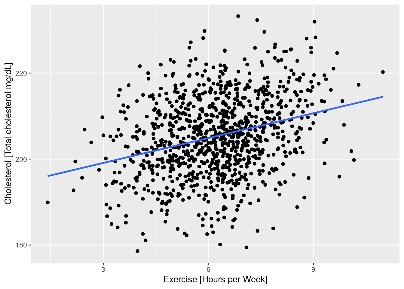

The results of an experiment, where x-axis represents how much exercise an individual does in hours, and y-axis represents cholestral measurment for the same individual.

Figure 1: The results of an experiment, where x-axis represents how much exercise an individual does in hours, and y-axis represents cholestral measurment for the same individual.

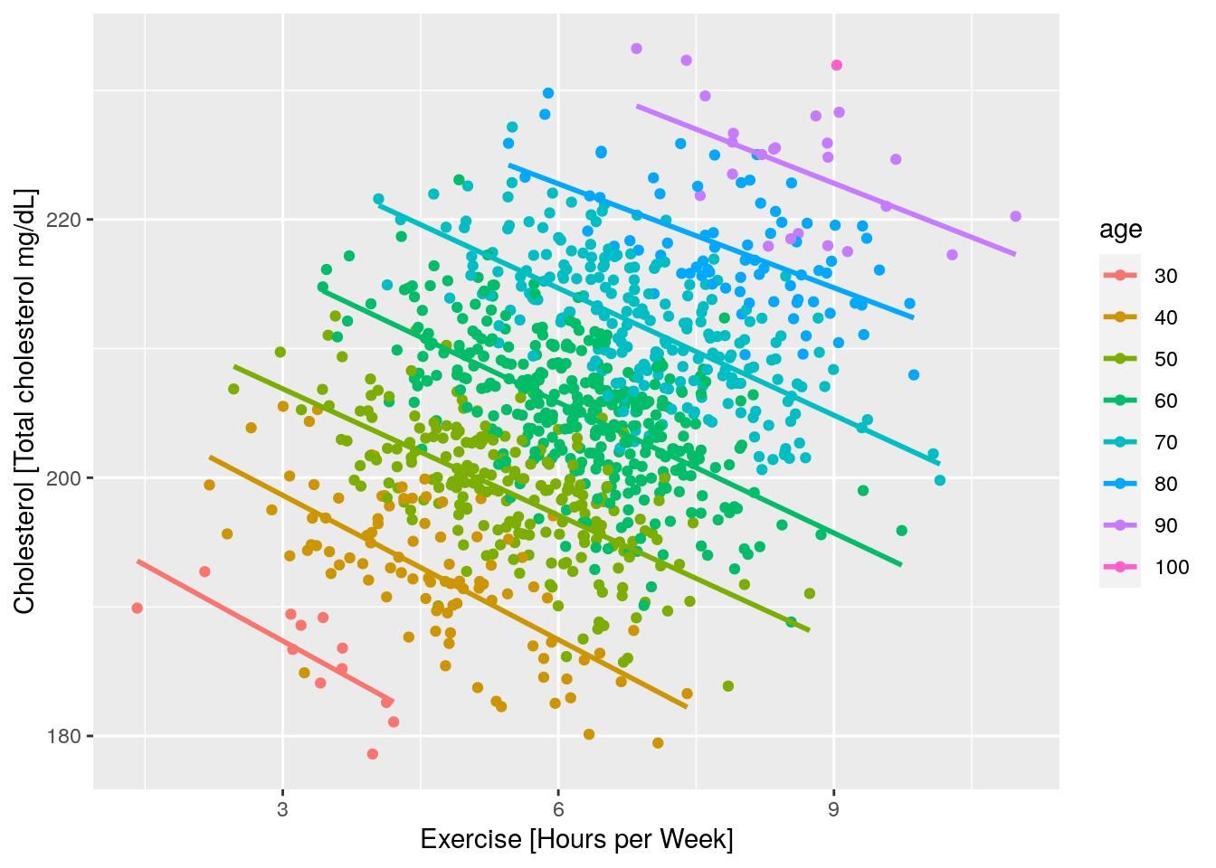
Figure 1 shows a positive correlation in an experiment that measures individuals’ exercise per week and cholesterol. At first glance, this seems absurd, but when we partition the data by another causal variable, this seems reasonable:

Figure 2: The same results as the experiment above, partioned by age

⊕(Also note, we have fabricated the data, although these relationships are quite plausible) Understanding the full causal story is essential. Without an entire causal narrative, we might recommend inappropriate interventions; for example, a doctor might prescribe less exercise to reduce cholesterol in the case above.

To deduce such causal stories, we need to apply the methodology of causal inference.

Structural Equation Models and Causal Graphs

A structural equation model (SEM) is a set of equations representing the relationship between variables. For example, the equations which generated the data from the Simpson’s paradox example, are given as: \[ \begin{align*} age &= U_1 \\ exercise &= \frac{1}{13}*age + U_2 \\ cholesteral &= -4*exercise + age + U_3 \end{align*} \] We can think of $U_1$, $U_2$, and $U_3$ as specific unobserved exogenous variables of an individual, which generate their endogenous variables (something like error terms).

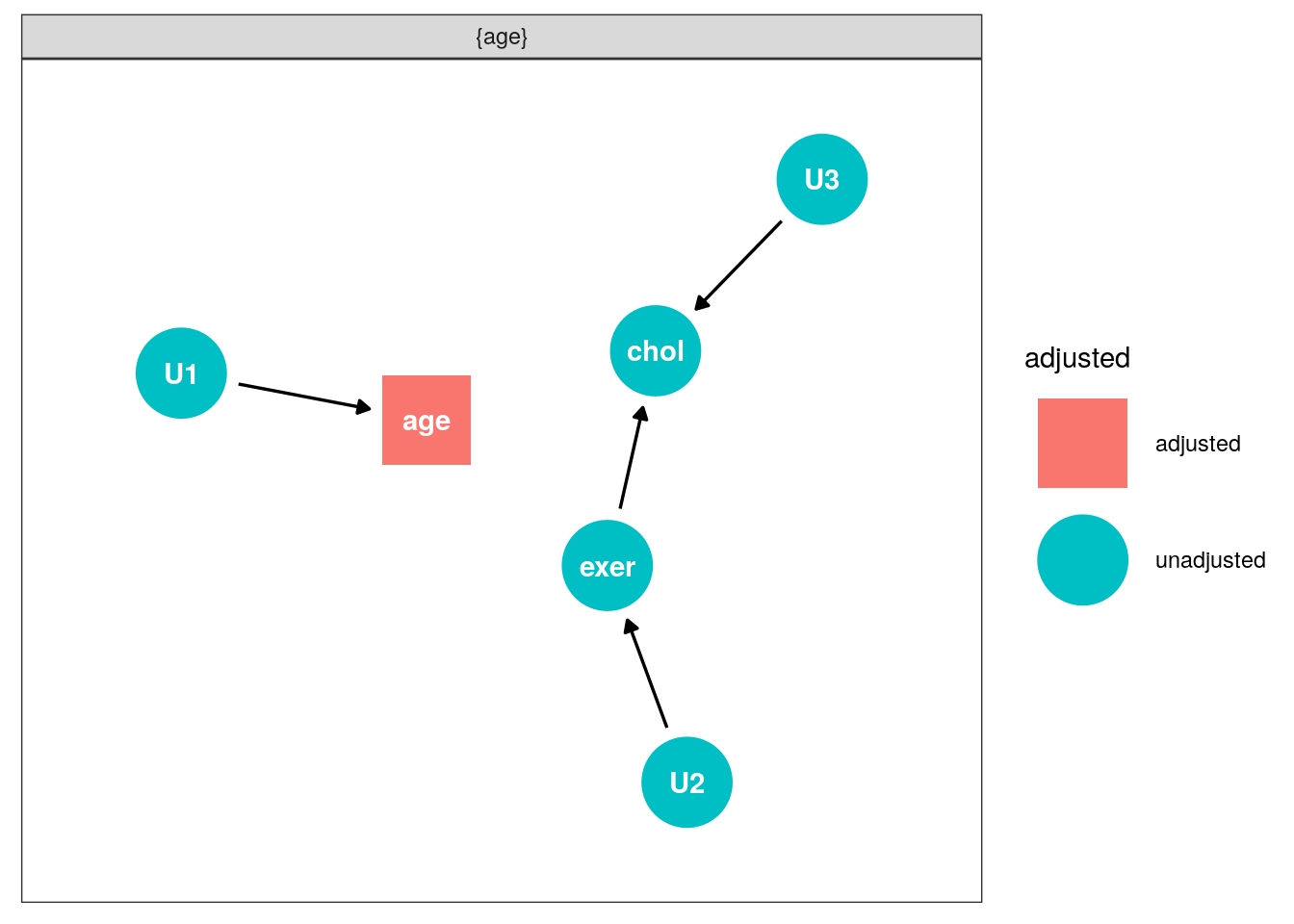
A causal graph is a DAG which describes the existence of relationships between variables in a model. An edge x -> y represents the relationship x directly causes y. Consequently, causal graphs can represent SEMs:

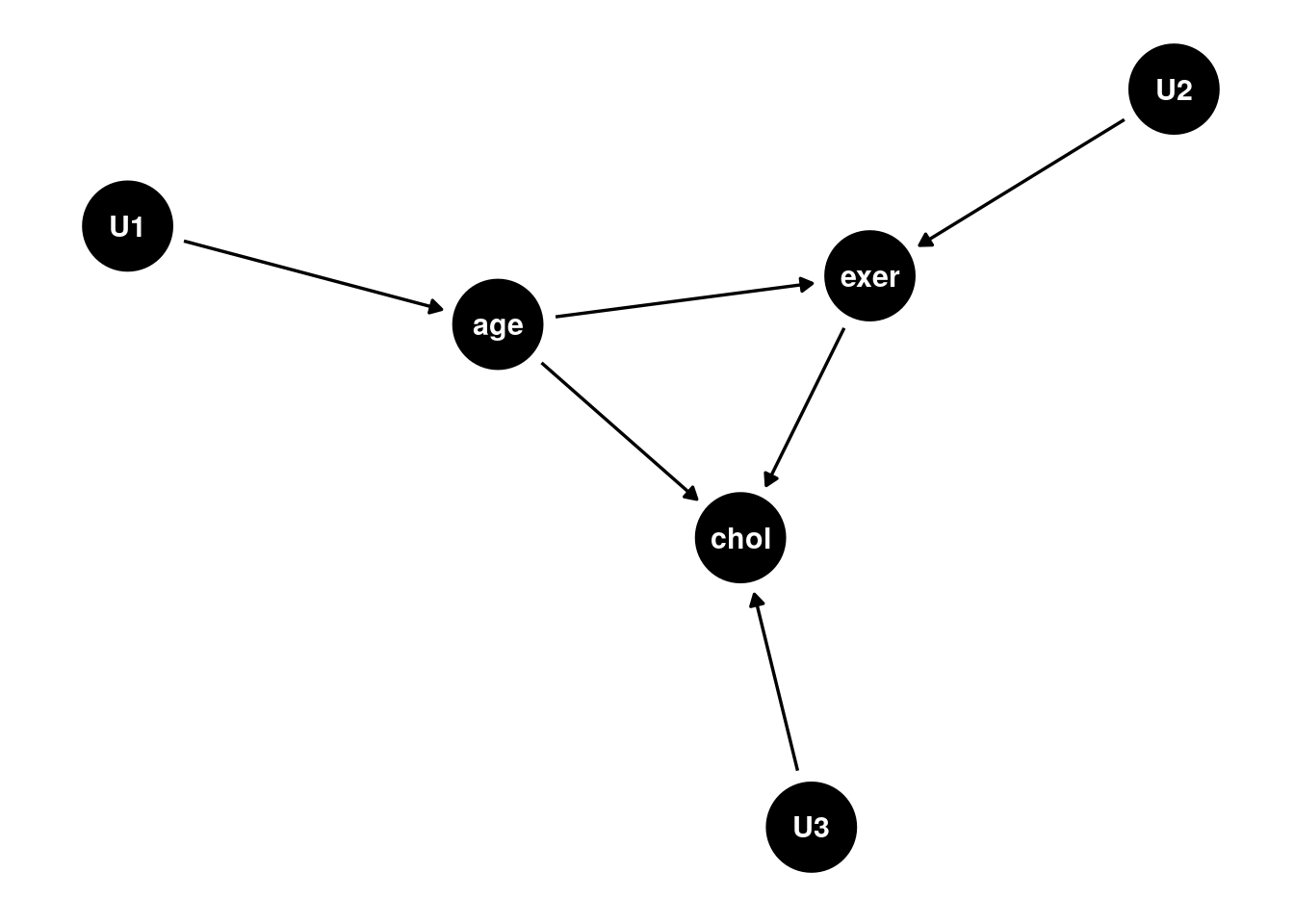
Indeed this graph shows how age confounds the effect of exercise on cholesterol.

Do-calculus

Pearl (1995) outline a method to remove this confounding (and other similar scenarios) using do-calculus. Outlining the specifics of do-calculus is beyond the scope of this blog post (but for interested readers, we suggest (Pearl, Glymour, and Jewell 2016)). In brief, do-calculus introduces the $do()$ operator, which acts as an intervention and fixes a variable to a particular constant. For example, consider a similar binary situation to the Simpson’s paradox example, where exer is a binary variable true if the individual is active, chol is a binary variable true if the individual has high cholesterol, and age is a binary variable true if the individual is over 60.

bin_simpsons_data <- simpsons_data %>%
  mutate(age = age > 60) %>% # Binarize the age, so those over 60 are True, and under 60 are False
  mutate(exer = exercise>mean(exercise)) %>% # Binarize the exercise level, so those above the average are True, and under are False
  mutate(chol = cholesteral>mean(cholesteral)) # Binarize the cholesteral level, so those above the average are True, and under are False

We ask the same experimental question; does exercise reduce cholesterol. A naive approach would be to compute the effect as $P(chol | exer = 1) - P(chol | exer = 0)=$ 0.168, where $P(chol | exer)$ is computed by filtering the data according to exer. Taking this approach, we would erroneously observe that the effect was positive since those who exercise more are also old and more likely to have high cholesterol.

The experimental best practice approach would be to perform a randomized controlled trial (RCT). A random selection of individuals are assigned to do a high exercise regiment and the others do a low exercise regiment (regardless of age). The RCT implicitly removes the natural tendency of exercise to vary with age and allows researchers to observe the causal effect of exercise on cholesterol. When using data generated in such a fashion, increases/decreases in the probability of having high cholesterol caused by exercise are given by $P_{RCT}(chol | exer = 1) - P_{RCT}(chol | exer = 0)$. This metric is known as the Average Causal Effect (ACE), sometimes called the Average Treatment Effect. Note that by conditioning on $exer=x$, with data generated by an RCT, researchers are essentially limiting the data used to estimate $P_{RCT}(chol | exer = x)$, to individuals who were forced to do an exercise regiment $x$. The do here represents forcing individuals to take an intervention value, regardless of their natural tendency, and this is captured by the $do()$ operator. In this case, $P(chol | do(exer = x)) = P_{RCT}(chol | exer = x)$, since the data was generated with an RCT. However, RCTs can be prohibitively expensive (both in time and money) and might not be necessary to tease out a causal effect.

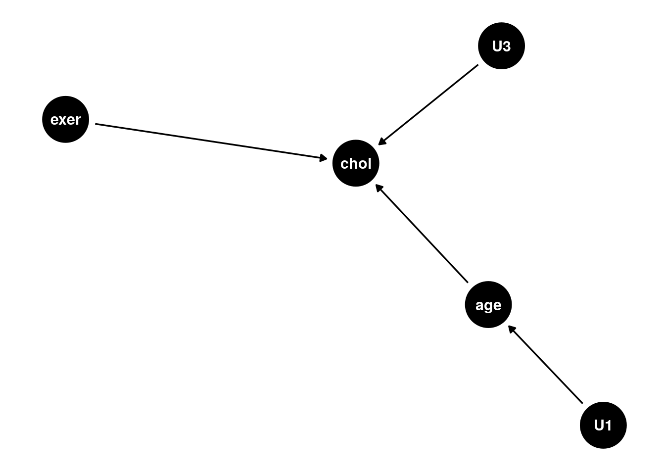
We would still like to estimate the ACE, $P(chol | do(exer = 1)) - P(chol | do(exer = 0))$, by using data that wasn’t generated from an RCT. By using the $do()$ operator here, we aim to disassociate exer from its natural tendency with age and effectively perform a graph surgery:

Pearl, Glymour, and Jewell (2016) provide an adjustment formula for just this scenario: \[ P(y|do(x)) = \sum_z \frac{P(X=x, Y=y, PA=z)}{P(X=x| PA=z)} \] where $X$ represents the variable we are acting on, $Y$ the variable we measure results from, and $PA$ the parents of $X$ and $Y$ or more generally any nodes that satisfy the back-door criterion (which we will introduce later). Note this allows us to derive the causal effect, as if we had generated data with an RCT, using only probabilities estimated from data not generated by an RCT.

As such we compute our ACE for the binary scenario:

# The Joint Distribution P(age, exer, chol) i.e. P(x,y,z)
p_aec <- bin_simpsons_data %>% 
  count(age, exer, chol) %>%
  mutate(freq = n/sum(n))

# The Marginal Distribution P(age) i.e. P(z)
p_a <- bin_simpsons_data %>% 
  count(age) %>%
  mutate(freq = n/sum(n))

# The Marginal Distribution P(age, exer) i.e. P(x, z)
p_ea <- bin_simpsons_data %>% 
  count(age, exer) %>%
  mutate(freq = n/sum(n))

# The Conditional Mariginal Distribution P(exer | age) i.e. P(x | z)
p_e_a <- p_a %>%  
  right_join(p_ea, by="age") %>%
  mutate(freq = freq.y/freq.x) %>%
  select(age, exer, freq)

# The Intervention Distribution P(chol | do(exer)) i.e. P(y | do(x))
probabilities <- data.table(p_aec %>% 
  left_join(p_e_a, by=c("age", "exer")) %>%
  mutate(freq = freq.x/freq.y) %>%
  select(age, exer, chol, freq) %>% 
  filter(chol) # We are only concerned with what cause high cholestral
)

# The average causal effect of exer on chol
ACE <- sum(probabilities[exer==T, freq]) - sum(probabilities[exer==F, freq])

This procedure leads to a negative ACE of -0.175, which shows the causal effect of going from high to low exercise on the probability of getting high cholesterol.

A natural question that follows from this example is, under what conditions can we use such adjustments to achieve an identifiable causal effect.

d-seperation

To understand common scenarios where the effect of variable $X$ on $Y$ is identifiable within a causal graph, we must first introduce the concept of d-separation, also known as blocking. A pair of variable $X$ and $Y$ are said to be blocked if they are conditionally independent, given a set of nodes $Z$. There are three graph types, which are essential for blocking:

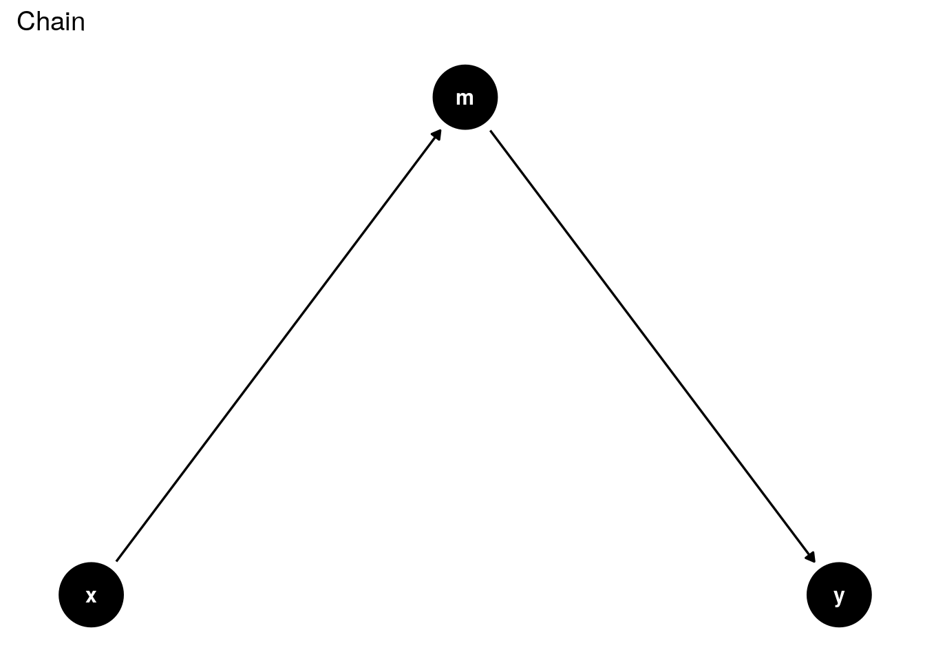
In the chain scenario, $X \sim Y$ is blocked by conditioning on $Z={M}$. This is sometimes refered to as the mediation scenario, which we will address further in the front-door criterion.

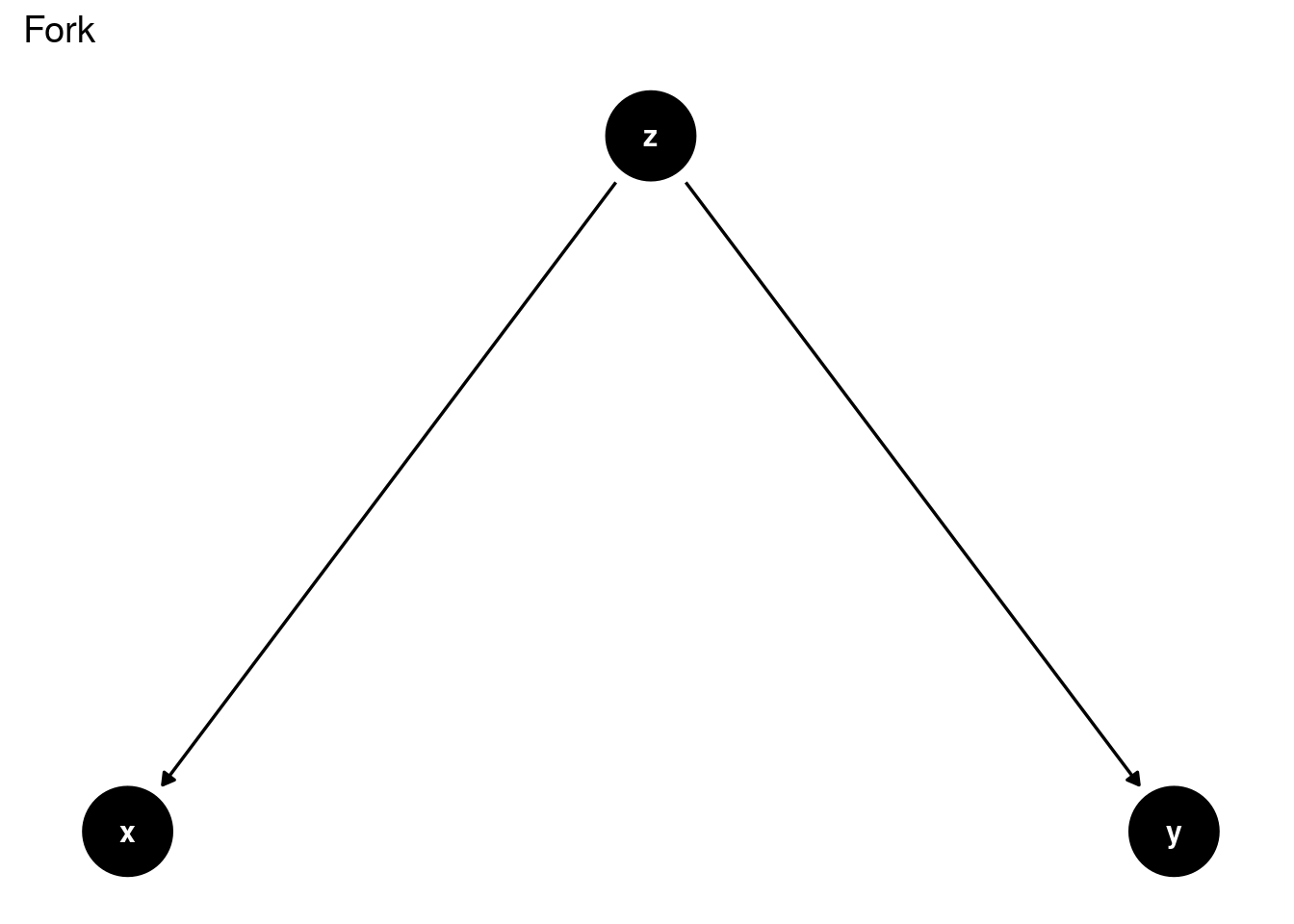
In the fork scenario, $X \sim Y$ is blocked by conditioning on $Z={Z}$. This is sometimes refered to as the confounder scenario, which is the situation in the simpson’s paradox example.

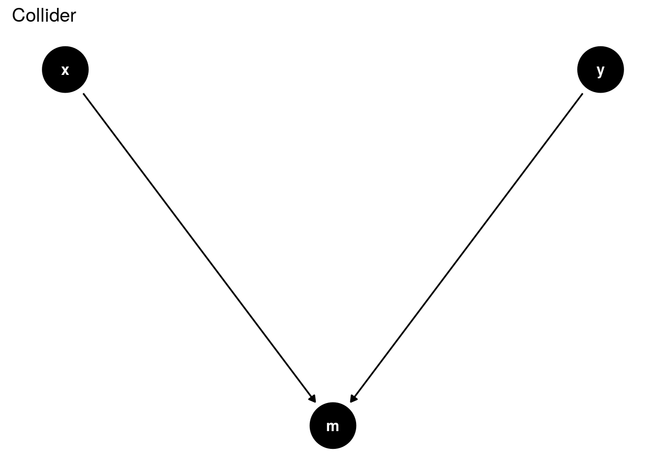
Finally, in the collider scenario, $X \sim Y$ is blocked by not conditioning on $Z={M}$. The idea that $X$ and $Y$, which are independent, to begin with, can become conditionally dependant is unintuitive. One way to think about this is that we are sharing information received from $ Y $ with $ X $ through $ M $ when we condition on $ M $. For a more thorough investigation into this phenomenon, refer to (Pearl, Glymour, and Jewell 2016).

A path is said to be blocked by $Z$ if it contains a chain or fork with its middle node in $Z$ or a collider with its middle node not in $Z$.

We are now ready to introduce the main criteria for which we can perform adjustments.

The Backdoor

Definition 1 (The Backdoor Criterion) A set of nodes $Z$, given a DAG $G$ and a pair of nodes $(X,Y)$, is said to satisfy the backdoor criterion if no node in $Z$ is a descendant of $X$, and $Z$ blocks all paths between $X$ and $Y$, which contain arrows into $X$.

If there exists are set of nodes why satisfy the backdoor criterion, then the effect of $X$ on $Y$ is identifiable and given by: \[ P(y|do(x)) = \sum_z \frac{P(X=x, Y=y, Z=z)}{P(X=x| Z=z)} \]

The backdoor criterion stops undue influence through the backdoor paths; it leaves direct paths between $X$ and $Y$, and it blocks spurious paths.

It is clear that { age } satisfies these conditions to be a backdoor adjustment set in the example above.

The Front-door

There are notably common scenarios where this doesn’t work. For example, consider a constructed causal mediation situation, as follows:

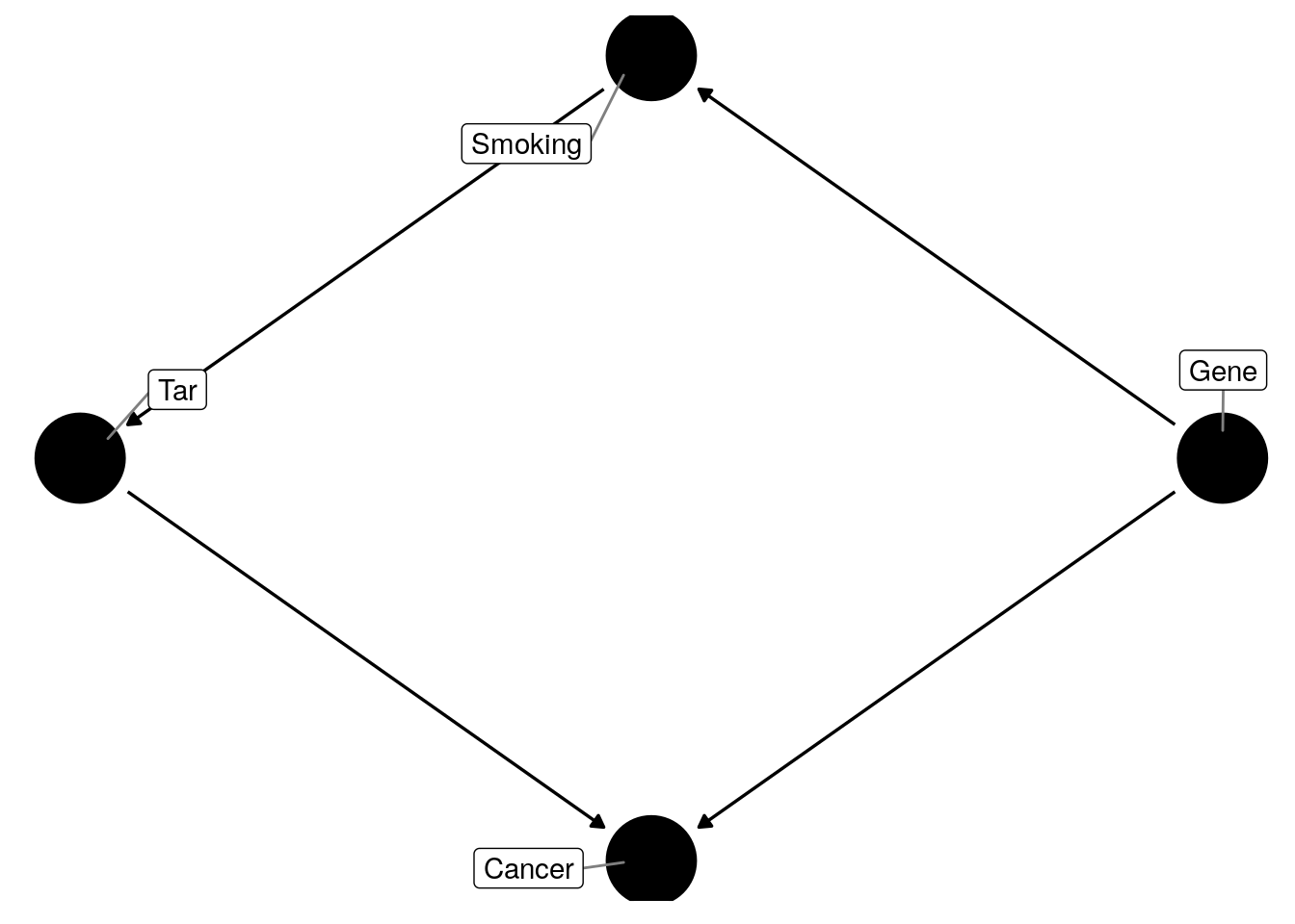
In this case we cannot use the backdoor criterion, to detect the effect of smoking on cancer because tar is a descendant of smoking, and there exists no direct link between smoking and cancer. We must use instead the frontdoor criterion:

Definition 2 (The Frontdoor Criterion) A set of nodes $Z$, given a DAG $G$ and a pair of nodes $(X,Y)$, is said to satisfy the frontdoor criterion if; $Z$ intercepts all direct paths from $X$ to $Y$, all paths between $X$ and $Z$ are blocked, and all backdoor paths between $Y$ and $Z$ are blocked by $X$.

If there exists are set of nodes $Z$ which satisfy the frontdoor criterion, and $P(x, z)>0$, then the effect of $X$ on $Y$ is identifiable and given by: \[ P(y|do(x)) = \sum_z P(z|x) \sum_{x^\prime} P(y|x^\prime, z)P(x^\prime) \] In our smoking scenario, we see that by adjusting for tar , we can observe the effect of smoking on cancer.

Conclusion

The above briefly outlines a core motivation for studying causal inference and causal stories. We summarise some of the underlying theory of causal inference and show practical methodology through the frontdoor and backdoor criterion for determining causal effects through entirely observational studies.

There are notable aspects of causal inference we have omitted from this taster. The most gaping is the lack of an explanation for the powerful tool of counterfactuals. We have only presented binary examples here (aside from our motivating example); however, perhaps the most common and useful causal inference application is to continuous examples using regression with linear models. Ultimately, we decided this was beyond causal inference taster’s scope and were more deserving of their own articles. Again, for the interested reader, we recommend Pearl, Glymour, and Jewell (2016), which adds links to many other resources.

Pearl, Judea. 1995. “Causal Diagrams for Empirical Research.” Biometrika 82 (4): 669–88.

Pearl, Judea, Madelyn Glymour, and Nicholas P Jewell. 2016. Causal Inference in Statistics: A Primer. John Wiley & Sons.

Simpson, Edward H. 1951. “The Interpretation of Interaction in Contingency Tables.” Journal of the Royal Statistical Society: Series B (Methodological) 13 (2): 238–41.